-
Basic commands
In order to have a package to use in R, you must install (once) and import (each .r file you want to use it in):
install.packages("")
library()Download CSV File
First, install downloader package:
Then in the file we want to:install.packages("downloader")
library(downloader)
url <- "https..."
filename <- "...csv"
download(url, destfile = filename)dplyr
There is also a great package for data manipulation and importation: dplyr
install.packages("dplyr")
library(dplyr)You can use the following:
- View(data) which lets you open a new tab to see the data
- filter() let's you look at just specific categories of data you want
- select() allows you to select and work with specific subset of data you want
- unlist() removes stuff from list format - becomes vector
- %>% is the inflix operator which works like a pipe, i.e., it passes the left hand side of the operator to the first argument of the right hand side of the operator. The point of it is to save time typing out data and graph changes
- basename(url) returns name.csv from a url
- summarize(aggregate_fn(column))
An example using a lot of these would be:
primate_sleep_list <- filter(m_sleep_df, order == "Primates") %>%
select(sleep_total) %>%
unlistYou can find my dplyr exercises here.
-
There are four panels in RStudio:
- top left source: where you open files and work on them
- bottom left console: where output is printed out and you can do operations
- top right environment/history: you can see what variables you have created
- bottom right help/plots/etc.: has all information and plots from the source/console
-
This great open source library that walks you through the basics of R. Here you can find a couple exercises I completed from the swirl tutorial. It goes through the following:
Basic building blocks
R has a lot of functions. As a coding language it is best used for mathematics and statistic calculations along with simulations.
The math operations are:
- <- : assigns a value to a variable
- + : adding
- - : subtracting
- / : dividing
- * : multiplying
- ^ : exponent
- %% : gives remainder
- remainder(num, divisor = #)
- sqrt() : square root
- abs() : absolute value
- mean()
- median()
- mode()
- c() : "concatenate"; creates a vector combining the objects within the brackets
For vector operations between vectors are done unit-to-unit if vectors are the same size, however, if vectors are different size, then the shorter vector is recycled until it is the same length as the longer one.
Workspace & files
Some commands that are useful for working on your system:
- getwd() : get working directory
- ls() : list objects in directory (variables created)
- list.files() : list files in directory
- args() : when used on a function name can let you see what arguments go into the function
- dir.create("name") : this let's you create a directory with a set "name"
- setwd("") : set which directory you want to work in
- file.create("name.R")
- file.rename("old.R", "new.R")
- file.remove("remove-name.R")
- file.copy("original.R", "copy.R")
- file.path("name.R")
- unlink("directory", recursive = TRUE) : deletes directory
Sequence of numbers
There are several different ways to get a sequence of numbers:
- : e.g. 1:3 gives us 1 2 3
- seq(#, #, by = increment, length = # of #s you want)
- seq(along.with = #) OR seq_along(#) : gives you a list of integers up until value inputted
- rep(#, times = how many times)
Vector
Atomic vector is a ve tor that contains exactly one data type (i.e. logical, character, integer, etc). List is a vector than cna contain multiple data types. Logical vector has TRUE or FALSE; it checks things using: NA!A, A|B, A&B, ==, !=, <=, >=, <, >. Character vectors double quotes are used to distinguish character objects.
Two useful vector things to know:
- LETTERS : is a predefined R variable for all the letters in the English alphabet.
- paste(vector, collapse = " ") : puts characters together from vector with a space in between; you can also specify something else to go inbetween each part of the vector using this function.
Missing Values
Working with missing values is a regular occurence for data. It is important to understand how to find out if there is missing data and also if to fill it and with what. Here are a couple of good to know functions when working with missing data:
- is.na(data_vector) : prints out TRUE or FALSE
- rnorm(#) : draws # of values from a standard normal distribution - which can be useful for inputting missing data
- sample(data, n) : lets you pull out random sample from your data - which can be useful for inputting missing data
- NA : null
- NaN : not a number
- Inf : infinity
Subsetting vectors
You can create subsets of vectors using vec[#:#] which uses index to pull out values from vector. We can also exclude indices: x[c(-2, -10)] or x[-c(2,10)].
You can also check if the vector is empty or not: is.na(vector) or !is.na(vector).
We can get the titles of the rows of a matrix or dataframe using names(matrix). And we can also check if two vectors are the same using identical(vector1, vector2) - which returns TRUE or FALSE.
Matrix and dataframes
Matrices can only contain one class of data, whereas, dataframes can contain more than one class. Here are some useful functions:
- length(df)
- attributes(df) : lists things like dimension, # of rows/columns, etc.
- matrix(data = , nrow = #, ncol = #) : creates a matrix with set row and columns
- cbind(vector, vector/matrix) : combines columns of two objects
- data.frame(vector/matrix, vector/matrix) : combines columns into dataframe
- colnames(df) <- list : let's you assign column names from a list
- rownames(df) <- list : let's you assign row names from a list
Neat fact is that you can access columns to perfomr aggregate functions by using df$column_name. For instance: sum(df$column_name).
Logic
Above there were some logic functions that were spoken of already. Here are some more:
- isTRUE(eq'n) : returns TRUE or FALSE
- xor(expression, expression) : only one expression needs to be true to return TRUE
- which(logical_vector) : returns true indices
- any(logical_vector) : returns TRUE if at least one component is true
- all(logical_vector) : returns TRUE is all of the components are true
Note that the number of typographical symbols is important:
- & : evaluates across a vector
- && : only evaluates the 1st member of a vector
Functions
Functions are created if you plan on reusing them. They are small pieces of reusable code. You can create a function in the same .R file or in a separate. After you have saved your function be sure to type submit() in your console to ensure you can use your function. Here is an example of one:
boring_function <- function(x) {
x}R has some very useful functions built in: lapply, sapply, vapply, and tapply - which I will go into more detail for.
Lapply and sapply
These are loop functions. They allow us to perform a function through a list.
lapply: applies a function to a list and returns a list.
sapply: applies a function to a list but returns values instead of list (i.e. a character list is returned). So for elements length one, it returns a vector. For elements that are the same sized vectors, it returns a matrix. If it cannot figure out what type it is, it returns a list.
Vapply and tapply
vapply: does same thing as sapply but allows you to specify format of results - thus speeding up the process for larger datasets.
tapply: allows the splitting of data by a specific value of some variable. An example:
this function takes the mean of animals separated by landmass.tapply(flags$animals, flags$landmass, mean)
Looking at data
Some useful dataframe functions are:
- head(df, #)
- tail(df, #)
- summary(df) : gives various details based on datatype per column
- dim(df)
- nrow(df)
- ncol(df)
- names(df) : column names - character vector
- str() : returns structure of df/function/etc.
- class(object)
- read.csv() : default stores it into a dataframe
- read.table() : also store in dataframe
- object.size(df) : size occupying memory
- unique(vector) : returns vector with duplicates removed
Simulation
Simulations are super useful for running experiments that are randomized to collect data. Here are the common functions used for simulations:
- sample(data, size, replace = FALSE, prob = NULL) : you can specify probability as a vector: c(0.3, 0.7) but it does not have to be known.
- replicate(number of times, distribution) : returns matrix of n trials of the specified distribution. You can also specify your own function instead of a distribution by using { }.
- colMeans(matrix) : takes mean of each column
-
We have a lot of different distributions/functions and variables that can be used for creating simulations. Here is a table that breaks down some of them:
r*
random functiond*
density functionp*
probability functionq*
quantile function*binom()
binomial distribution (R.V.)rbinom() dbinom() pbinom() qbinom() *norm()
normal distribution (R.V.)*pois()
poisson distribution (R.V.)*exp()
exponential distribution (R.V.)*chisq()
chi-square distribution (R.V.)*gamma()
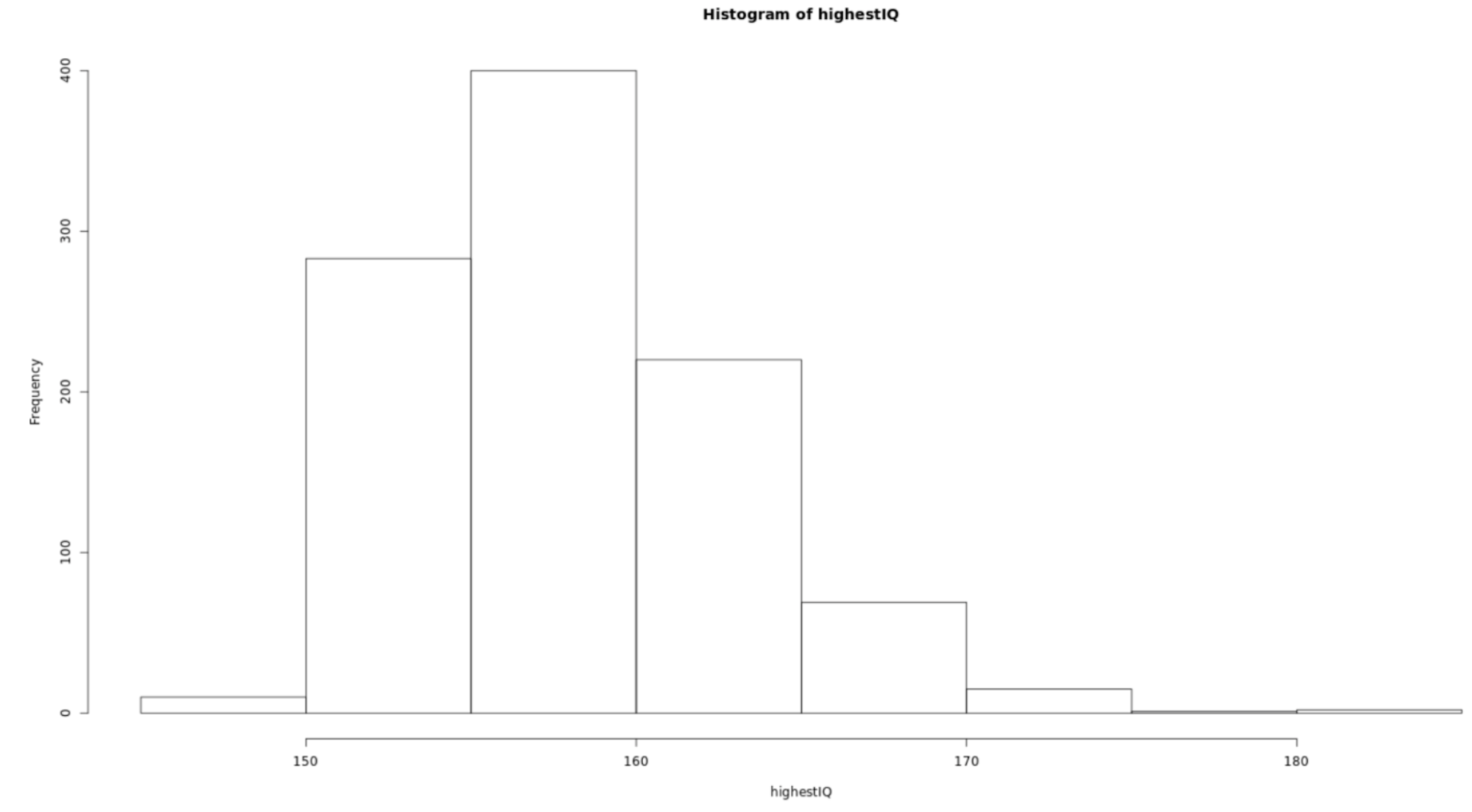
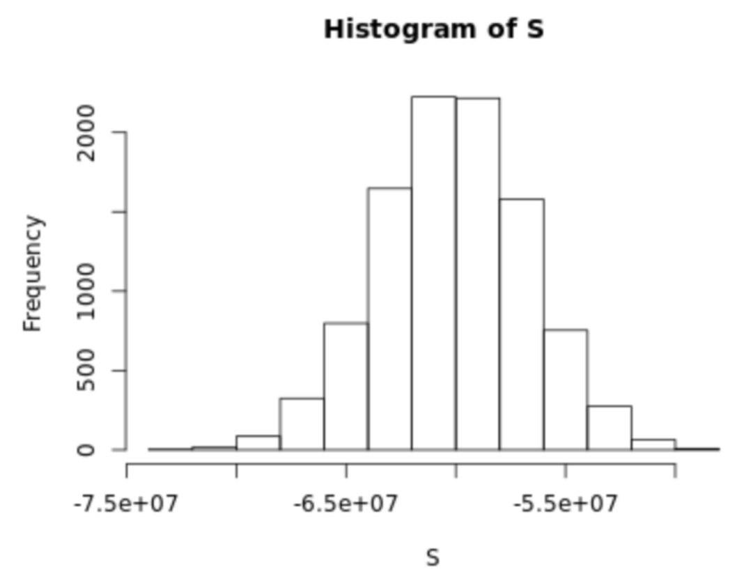
gamma distribution (R.V.) - hist(data) : creates histogram of data - more on visualization in a different course.
Dates and time
Dates and times are represented by POSIXct (the number of dats.# of seconds since 1970-01-01) and POSIXlt (list of seconds, minutes, hour, etc.). Some useful function to know:
- Sys.Date() : days since 1970-01-01
- Sys.time() : time in POSIXlt formate
- weekdays()
- months()
- quarters()
- strtime() : ?strptime gives you a list of variablwe to specify which correspons to what (e.g. %B is the full month name)
- difftime(time1, time 2, units="days") : gives the number of days between the two times
Base graphics
As mentioned before this we will go over in more detail in the visualization course section later on. Here are some basic functions to get us started:
- data(data) : loads dataframe with data given
-
plot(data) : creates scatterplot; can access parameters of plot using ?par. An example of a basic scatterplot:
plot(x=df$name, y=df$name, xlab = "xlabel", xlim = c(#beginx, #endx), ylab = "ylabel", main = "Main Title", sub = "subtitle", col = number representing color for plot)
- boxplot()



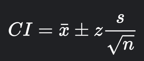
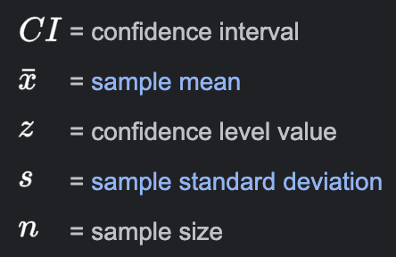
 .
.

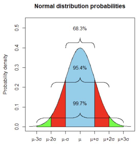
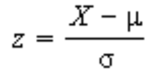
 . While the equation to convert from a random variable (X) to the normal (Z) is given by











 . The OPS metric gives the most weight to:
